Adrian Cockroft poses an interesting question in, Who monitors the monitoring systems? He states, The first thing that would be useful is to have a monitoring system that has failure modes which are uncorrelated with the infrastructure it is monitoring. ... I don’t know of a specialized monitor-of-monitors product, which is one reason I wrote this blog post.
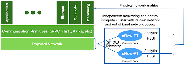
This article offers a response, describing how to introduce an uncorrelated monitor-of-monitors into the data center to provide real-time visibility that survives when the primary monitoring systems fail.
Standardizing on a small set of communication primitives (gRPC, Thrift, Kafka, etc.) simplifies the creation of large scale distributed services. The communication primitives abstract the physical network to provide reliable communication to support distributed services running on compute nodes. Monitoring is typically regarded as a distributed service that is part of the compute infrastructure, relying on agents on compute nodes to transmit measurements to scale out analysis, storage, automation, and presentation services.
System wide failures occur when the network abstraction fails and the limitations of the physical network infrastructure intrude into the overlaid monitoring, compute, storage, and application services. Physical network service failure is the Achilles heel of distributed compute infrastructure since the physical network is the glue that ties the infrastructure together.
However, the physical network is also a solution to the monitoring problem, providing an independent uncorrelated point of observation that has visibility into all the physical network resources and the services that run over them.
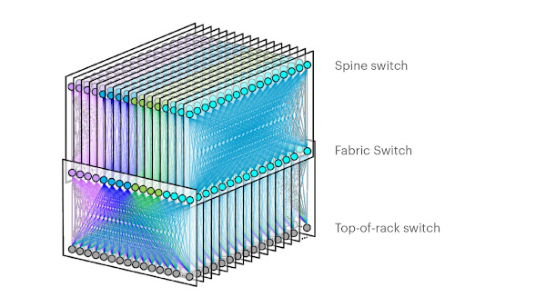
Reinventing Facebook’s data center network describes the architecture of a data center network. The network is a large distributed system made up of thousands of hardware switches and the tens of thousands of optical links that connect them. The network can route trillions of packets per second and has a capacity measured in Petabits/second.
The industry standard sFlow measurement system, implemented by all major data center network equipment vendors, is specifically designed to address the challenge of monitoring large scale switched networks. The sFlow specification embeds standard instrumentation into the hardware of each switch, making monitoring an integral part of the function of the switch, and ensuring that monitoring capacity scales out as network size increases.
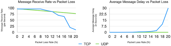
UDP vs TCP for real-time streaming telemetry describes how sFlow uses UDP to transport measurements from the network devices to the analytics software in order to maintain real-time visibility during network congestion events. The graphs from the article demonstrate that the different transport characteristics of UDP and TCP decouple the physical network monitoring system from the primary monitoring systems which typically depend on TCP services.
The diagram at the top of this article shows the elements of an sFlow monitoring system designed to provide independent visibility into large scale data center network infrastructure.
Each network device can be configured to send sFlow telemetry to at least two destinations. In the diagram two independent instances of the sFlow-RT real-time analytics engine are deployed on two separate compute nodes, each receiving its own stream of telemetry from all devices in the network. Since both sFlow-RT instances receive the same telemetry stream, they independently maintain copies of the network state that can be separately queried, ensuring availability in the event of a node failure.
Note: Tollerance to packet loss allows sFlow to be sent inband to reduce load on out-of-band management networks without significant loss of visibility.
Scalability is ensured by sFlow's scale out hardware-based instrumentation. Leveraging the collective capability of the distributed instrumentation allows each sFlow-RT instance to monitor the current state of the entire data center network.
Tuning Performance describes how to optimize sFlow-RT performance for large scale monitoring.
The compute nodes hosting sFlow-RT instances should be physically separate from production compute service and have an independent network with out of band access so that measurements are available in cases were network performance issues have disrupted the production compute service.
This design is intentionally minimalist in order to reliably deliver real-time visibility during periods of extreme network congestion when all other systems fail.
In Failure Modes and Continuous Resilience, Adrian Cockroft states, The first technique is the most generally useful. Concentrate on rapid detection and response. In the end, when you’ve done everything you can do to manage failures you can think of, this is all you have left when that weird complex problem that no-one has ever seen before shows up!
With the state of the network stored in memory, each sFlow-RT instance provides an up to the second view of network performance with query response times measured in milliseconds. Queries are optimized to quickly diagnose network problems:
Detect network congestion
Identify traffic driving congestion
Locate control points to mitigate congestion
Real-time traffic analytics can drive automated remediation for common classes of problem to rapidly restore network service. Automated responses include:
Filtering out DDoS traffic
Shed non-essential services
Re-routing traffic
Shaping traffic
Of course, reliable control actions require an out-of-band management network so that controls can be deployed even if the production network is failing. Once physical network congestion problems have been addressed, restored monitoring services will provide visibility into production services and allow normal operations to resume. Real-time physical network visibility allows automated control actions to resolve physical network congestion problems within seconds so that there is negligible impact on the production systems.
Physical network visibility has utility beyond addressing extreme congestion events, feeding physical network flow analytics into production monitoring systems augments visibility and provides useful information for intrusion detection, capacity planning, workload placement, autoscaling, and service optimization. In addition, comparing the independently generated flow metrics profiling production services with the metrics generated by the production monitoring systems provides an early warning of monitoring system reliability. Finally, the low latency of network flow metrics are a leading indicator of performance that can be used to improve the agility of production monitoring and control.
The sFlow-RT real-time analytics platform receives a continuous telemetry stream from sFlow Agents embedded in network devices, hosts and applications and converts the raw measurements into actionable metrics, accessible through open APIs, see Writing Applications.
Application development is greatly simplified if you can emulate the infrastructure you want to monitor on your development machine. Mininet flow analytics, Mininet dashboard, and Mininet weathermap describe how to use the open source Mininet network emulator to simulate networks and generate a live stream of standard sFlow telemetry data.
This article describes how to use Docker containers as a development platform. Docker Desktop provides a convenient method of running Docker on Mac and Windows desktops. These instructions assume you have already installed Docker.
Run the following command in the original terminal to initiate a test and generate traffic:
docker run --rm sflow/iperf3 -c host.docker.internal
You should immediately see a spike in traffic like that shown in the Flow Browser screen capture. See RESTflow for an overview of the sFlow-RT flow analytics architecture and Defining Flows for a detailed description of the options available when defining flows.
Another option is to replay sFlow telemetry captured in the form of a PCAP file. The Fabric View application contains an example that can be extracted:
The above command retrieves metrics for all the hosts in Prometheus export format. Prometheus exporter describes how run the Prometheus time series database and build Grafana dashboards using metrics retrieved from sFlow-RT. Flow metrics with Prometheus and Grafana extends the example to include packet flow data. InfluxDB 2.0 shows how to import and query metrics using InfluxDB.
It only takes a few minutes to try out these examples. Work through Writing Applications to learn about the capabilities of the sFlow-RT analytics engine and how to package applications. Publish applications on GitHub and use the sflow/sflow-rt Docker image to deploy them in production. Join the sFlow-RT Community to ask questions and post information new applications.
Monitoring Linux services describes how the open source Host sFlow agent exports metrics from services launched using systemd, the default service manager on most recent Linux distributions. In addition, the Host sFlow agent efficiently samples network traffic using Linux kernel capabilities: PCAP/BPF, nflog, and ulog.
This article describes a recent extension to the Host sFlow systemd module, mapping sampled traffic to the individual services the generate or consume them. The ability to color traffic by application greatly simplifies service discovery and service dependency mapping; making it easy to see how services communicate in a multi-tier application architecture.
The following /etc/hsflowd.conf file configures the Host sFlow agent, hsflowd, to sampling packets on interface eth0, monitor systemd services and mark the packet samples, and track tcp performance:
sflow {
  collector { ip = 10.0.0.70 }
  pcap { dev = eth0 }
  systemd { markTraffic = on }
  tcp { }
}
The diagram above illustrates how the Host sFlow agent is able to efficiently monitor and classify traffic. In this case both the Host sFlow agent and an Apache web server are are running as services managed by systemd. A network connection , shown in red, to the HTTP service. In this case, configuring the pcap module to monitor interface eth0 on the server programs a Berkeley Packet Filter (BPF) that randomly samples packets in the Linux kernel and provides copies (shown as the dotted red line) to the Host sFlow agent. In addition, the Host sFlow agent queries systemd to obtain a list of running services and the resources allocated to them. Further Linux kernel tables are queried to identify the network sockets that were opened by each service.
The Host sFlow then attaches an additional record to exported packet samples to indicate the services generating or consuming the packets:
/* Traffic source/sink entity reference */
/* opaque = flow_data; enterprise = 0; format = 2210 */
/* Set Data source to all zeroes if unknown
struct extended_entities {
 sflow_data_source_expanded src_ds;    /* Data Source associated with
                                          packet source */
 sflow_data_source_expanded dst_ds;    /* Data Source associated with
                                          packet destination */
}
Note: The data source references point to the performance metrics exported by the systemd module, see Monitoring Linux services.
Finally, enabling the tcp module adds delay, retransmit, loss, and reordering information to the sampled packet, see Network performance monitoring.
The screen capture above shows network traffic colored by service name. The chart colors traffic associated with the httpd.service in blue, remote login traffic associated with the sshd.service in red, BGP traffic associated with the bird.service in gold, and traffic to the inmsfd.service in green.
The chart was generated using the open source Flow Trend application running on the sFlow-RT real-time analytics platform. The chart is the result of the following flow definition:
host:[or:dssource:dsdestination]:vir_host_name
The host: function is used to join information from the sampled flow with telemetry reported for each of the services. Additional keys can be added to the flow definition to break out the traffic by network addresses, quality of service, or any of the many properties reported by sFlow, see Defining Flows for additional information.
Networking on the host has been referred to as the "Goldilocks Zone" because the host provides context that is unavailable in network switches and routers. The sFlow standard defines measurements that network, host, and application entities send in a continuous telemetry stream to analytics software that can combine the data to provide a comprehensive end-to-end view of activity, see sFlow Host Structures.
The screen capture from the Ganglia monitoring tool shows metrics for services running on a Linux host. Monitoring Linux services describes how the open source Host sFlow agent has been extended to export standard Virtual Node metrics from services running under systemd. Ganglia already supports these standard metrics and the article Using Ganglia to monitor virtual machine pools describes the configuration steps needed to enable this feature.
Mainstream Linux distributions have moved to systemd to manage daemons (e.g. httpd, sshd, etc.). The diagram illustrates how systemd runs each daemon within its own container so that it can maintain tight control of the daemon's resources.
This article describes how to use the open source Host sFlow agent to gather telemetry from daemons running under systemd.
Host sFlow systemd monitoring exports a standard set of metrics for each systemd service - the sFlow Host Structures extension defines metrics for Virtual Nodes (virtual machines, containers, etc.) that are used to export Xen, KVM, Docker, and Java resource usage. Exporting the standard metrics for systemd services provides interoperability with sFlow analyzers, allowing them to report on Linux services using existing virtual node monitoring capabilities.
While running daemons within containers helps systemd maintain control of the resources, it also provides a very useful abstraction for monitoring. For example, a single service (like the Apache web server) may consist of dozens of processes. Reporting on container level metrics abstracts away the per-process details and gives a view of the total resources consumed by the service. In addition, service metadata (like the service name) provides a useful way of identifying and grouping services, for example, making it easy to report on total CPU consumed by the web service across a pool of servers.
Next, enable the systemd module by adding the highlighted line in the /etc/hsflowd.conf file:
sflow{
  collector{ ip=10.0.0.1 }
  systemd{}
}
This is a minimal configuration that sends sFlow telemetry to a collector running on host 10.0.0.1. The Host sFlow agent is capable of gathering an extensive set of network, system and application level metrics. See Configuring Host sFlow for Linux for a full set of options.
The Host sFlow agent will automatically detect when cgroup accounting has been enabled. However, if cgroup accounting hasn't been enabled, it is still able to compute and export statistics, although it might miss contributions from short lived processes.
Once the agents have been configured, verify that sFlow telemetry is being received at the collector using sflowtool. The simplest way to run sflowtool is using Docker:
docker run -p 6343:6343/udp sflow/sflowtool
The following output shows the statistics exported for the apache2 service:
Custom metrics with Cumulus Linux describes how to extend the set of metrics exported by the sFlow agent and used the export of BGP metrics as an example. This article demonstrates how environmental metrics (power supplies, temperatures, fan speeds etc.) can be exported.
The smonctl command can be used to dump sensor data as JSON formatted text:
Note: Make sure the following line is uncommented in the /etc/hsflowd.conf file in order to receive custom metrics. If the file is modified, restart hsflowd for the changes to take effect.
jsonPort = 36343
Adding the following cron entry runs the script every minute:
This example requires Host sFlow version 1.28.3 or later. This is newer than the version of Host sFlow that currently ships with Cumulus Linux 2.5.5. However, Cumulus Linux is an open platform, so the software can be compiled from sources in just the same way you would on a server:
sudo sh -c 'echo "deb http://ftp.us.debian.org/debian wheezy main contrib" > /etc/apt/sources.list.d/deb.list'
sudo apt-get update
sudo apt-get install gcc make libc-dev
wget https://github.com/sflow/host-sflow/archive/v1.28.3.tar.gz
tar -xvzf v1.28.3.tar.gz
cd host-sflow-1.28.3
make CUMULUS=yes
make deb CUMULUS=yes
sudo dpkg -i hsflowd_1.28.3-1_ppc.deb
The sFlow-RT chart at the top of this page shows a trend chart of the environment metrics. Each metrics has been constructed as a percentage, so they can all be combined on the chart.
While custom metrics are useful, they don't capture the semantics of the data and will vary in form and content. In the case of environmental metrics, a standard set of metrics would add significant value since many different types of device include environmental sensors and a common set of measurements from all networked devices would provide a comprehensive view of power, temperature, humidity, and cooling. Anyone interested in developing a standard sFlow export for environmental metrics can contribute ideas on the sFlow.org mailing list.
Cumulus Networks, sFlow and data center automation describes how Cumulus Linux is monitored using the open source Host sFlow agent that supports Linux, Windows, FreeBSD, Solaris, and AIX operating systems and KVM, Xen, XCP, XenServer, and Hyper-V hypervisors, delivering a standard set of performance metrics from switches, servers, hypervisors, virtual switches, and virtual machines.
Host sFlow version 1.28.3 adds support for Custom Metrics. This article demonstrates how the extensive set of standard sFlow measurements can be augmented using custom metrics.
Recent releases of Cumulus Linux simplify the task by making machine readable JSON a supported output in command line tools. For example, the cl-bgp tool can be used to dump BGP summary statistics:
A more interesting way to consume this data is using sFlow-RT. The diagram above shows a leaf and spine network built using CumuluxVX virtual machines that was used for a Network virtualization visibility demo. Installing the bgp_sflow.py script on each switch adds centralized visibility into fabric wide BGP statistics.
For example, the following sFlow-RT REST API command returns the total bgp messages sent and received summed across all switches:
The custom metrics are fully integrated with all the other sFlow metrics, for example, the following query returns the host_name, bgp-as and load_one metrics associated with bgp-router-id 192.168.0.80:
Software, documentation, applications, and community support is available on sFlow-RT.com. For example, the sFlow-RT Fabric View application shown in the screen capture calculates and displays fabric wide traffic analytics.
The GitHub gmond-proxy project demonstrates how a simple proxy can be used to map metrics retrieved through a REST API into Ganglia's gmond TCP protocol.
The diagram shows the elements of the Ganglia monitoring system. The Ganglia server contains runs the gmetad daemon that polls for data from gmond instances and stores time series data. Trend charts are presented through the web interface. The transparent gmond-proxy replaces a native gmond daemon and delivers metrics in response to gmetad's polling requests.
The following commands install the proxy on the sFlow collector - an Ubuntu 14.04 system that is already runnig sFlow-RT:
Next edit the /etc/ganglia/gmetad.conf file and configure the proxy as a data source:
data_source "my cluster" sflow-rt
Restart the Apache and gmetad daemons:
sudo service gmetad restart
sudo service apache2 restart
The Ganglia web user interface, shown in the screen capture, is now available at http://server/ganglia/
Ganglia natively supports sFlow, so what are some of the benefits of using the proxy? Firstly, the proxy allows metrics to be filtered, reducing the amount of data logged and increasing the scaleability of the Ganglia collector. Secondly, sFlow-RT generates traffic flow metrics, making them available to Ganglia. Finally, Ganglia is typically used in conjunction with additional monitoring tools that can all be driven using the analytics stream generated by sFlow-RT.
The diagram above shows how the sFlow-RT analytics engine is used to deliver metrics and events to cloud based and on-site DevOps tools, see: Cloud analytics, InfluxDB and Grafana, Metric export to Graphite, and Exporting events using syslog. There are important scaleability and cost advantages to placing the sFlow-RT analytics engine in front of metrics collection applications as shown in the diagram. For example, in large scale cloud environments the metrics for each member of a dynamic pool are not necessarily worth trending since virtual machines are frequently added and removed. Instead, sFlow-RT can be configured to track all the members of the pool, calculate summary statistics for the pool, and log summary statistics. This pre-processing can significantly reduce storage requirements, reduce costs and increase query performance.
The flow-graph application, shown above, generates a real-time graph of communication between hosts. The application uses a simple sFlow-RT script to track associations between hosts based on their communication patterns and plots the results using the vis.js dynamic, browser based visualization library. This example can be modified to track different types of relationship and extended to incorporate other popular data visualization libraries such as D3.js.
The dashboard-example includes representative real-time metric and top flows trend charts. The example uses the jQuery-UI library to build build a simple tabbed interface. This example can be extended to build groups of custom charts.
The top-flows application supports the definition of custom flows and tracks the largest flows in a continuously updating table.
Each of the examples has a server-side component that uses sFlow-RT's script API to collect, analyze, and export measurements. An HTML5 client side user interface connects to the server and presents the data.
The sFlow-RT analytics engine is a highly scaleable platform for processing sFlow measurements from physical and virtual network switches, servers, virtual machines, Linux containers, load balancers, web and application servers, etc. The analytics capability can be applied to a wide range of SDN and DevOps use cases - many of which have been described on this blog. Application support provides a simple way for vendors, researchers, and developers to distribute solutions.
Open Virtual Network (OVN) is an open source network virtualization solution built as part of the Open vSwitch (OVS) project. OVN provides layer 2/3 virtual networking and firewall services for connecting virtual machines and Linux containers.
OVN is built on the same architectural principles as VMware's commercial NSX and offers the same core network virtualization capability — providing a free alternative that is likely to see rapid adoption in open source orchestration systems, Mirantis: Why the Open Virtual Network (OVN) matters to OpenStack.
This article uses OVN as an example, describing a testbed which demonstrates how the standard sFlow instrumentation build into the physical and virtual switches provides the end-to-end visibility required to manage large scale network virtualization and deliver reliable services.
Open Virtual Network
The Northbound DB provides a way to describe the logical networks that are required. The database abstracts away implementation details which are handled by the ovn-northd and ovn-controllers and presents an easily consumable network virtualization service to orchestration tools like OpenStack.
The purple tables on the left describe a simple logical switch LS1 that has two logical ports LP1 and LP2 with MAC addresses AA and BB respectively. The green tables on the right show the Southbound DB that is constructed by combining information from the ovn-controllers on hypervisors HV1 and HV2 to build forwarding tables in the vSwitches that realize the virtual network.
Docker, OVN, OVS, ECMP Testbed
The diagram shows the virtual testbed that was created using virtual machines running under VirtualBox:
Physical Network The recent release of Cumulus VX by Cumulus Networks makes it possible to build realistic networks out of virtual machines. In this case we built a two-spine, two-leaf network using VirtualBox that provides L3 ECMP connectivity using BGP as the routing protocol, a configuration that is very similar to that used by large cloud providers. The green virtual machines leaf1, leaf2, spine1 and spine2 comprise the ECMP network.
ServersServer 1,Server 2 and the Orchestration Server virtual machines are ubuntu-14.04.3-server installations. Server 1 and Server 2 are connected to the physical network with addresses 192.168.1.1 and 192.168.2.1 respectively that will be used to form the underlay network. Docker has been installed on Server 1 and Server 2 and each server has two containers. The containers on Server 1 have been assigned addresses 172.16.1.1/00:00:00:CC:01:01 and 172.16.1.2/00:00:00:CC:01:02 and the containers on Server 2 have been assigned addresses 172.16.2.1/00:00:00:CC:02:01, 172.16.2.2/00:00:00:CC:02:02.
Virtual NetworkOpen vSwitch (OVS) was installed from sources on Server 1 and Server 2 along with ovn-controller daemons. The ovs-northd daemon was built and installed on the Orchestration Server. A single logical switch sw0 has been configured that connects the server1-container2 (MAC 00:00:00:CC:01:02) to server2-container2 (MAC 00:00:00:CC:02:02).
Management Network The out of band management network shown in orange is a VirtualBox bridged network connecting management ports on the physical switches and servers to the Orchestration Server.
Pinging between Server 1, Container 2 (172.16.1.2) and Server 2, Container 2 (172.16.2.2) verifies that the logical network is operational.
Visibility
Enabling sFlow instrumentation in the testbed provides visibility into the physical and virtual network and server resources associated with the logical network.
Most physical switches support sFlow. With Cumulus Linux, installing the Host sFlow agent enables the hardware support for sFlow in the bare metal switch to provide line rate monitoring on every 1, 10, 25, 40, 50 and 100 Gbit/s port. Since Cumulus VX isn't a hardware switch the Host sFlow agent makes use of the Linux iptables/nflog capability to monitor traffic.
Host sFlow agents are installed on Server 1 and Server 2. These agents stream server, virtual machine, and container metrics. In addition, the Host sFlow agent automatically enables the sFlow in Open vSwitch which in turn exports traffic flow, interface counter, resource and tunnel encap/decap information.
The sFlow data from the leaf1, leaf2, spine1, spine2, server1 and server2 is transmitted over the management network to sFlow-RT real-time analytics software running on the Orchestration Server.
A difficult challenge in managing large scale cloud infrastructure is rapidly identifying overloaded resources (hot spots), for example:
Congested network link between physical switches
Poorly performing virtual switch
Overloaded server
Overloaded container / virtual machine
Oversubscribed service pool
Distributed Denial of Service (DDoS) attack
DevOps
Identifying an overloaded resource is only half the solution - the source of the load must also be found so that corrective action can be taken. This process of identifying and curing overloaded resources is critical to delivering on service level agreements. The scale and complexity of the infrastructure demands that this process be automated so that performance problems are quickly identified and immediately addressed.
The sFlow-RT analytics platform is designed with automation in mind, providing REST and embedded script APIs that facilitate metrics driven control actions. The following examples use the sFlow-RT REST API to demonstrate the type of data available using sFlow.
Congested network link between physical switches
The following query find the busiest link in the fabric based on sFlow interface counters:
Now we know that interface swp2 on switch leaf1 is the busy link, the next step is identifying the traffic flowing on the link by creating a flow definition (see RESTflow):
curl -H "Content-Type:application/json" -X PUT -d '{"keys":"macsource,macdestination,ipsource,ipdestination,stack","value":"bytes"}' http://10.0.0.86:8008/flow/test1/json
Now that a flow has been defined, we can query the new metric to see traffic on the port:
We can see that the traffic is a Geneve tunnel between Server 2 (192.168.2.1) and Server 1 (192.168.1.1) and that it is carrying encapsulated ICMP traffic. At this point, an additional flow can be created to find the sources of traffic in the virtual overlay network (see Down the rabbit hole).
The following flow definition takes the data from the physical switches and examines the tunnel contents:
curl -H "Content-Type:application/json" -X PUT -d '{"keys":"ipsource,ipdestination,genevevni,macsource.1,host:macsource.1:vir_host_name,macdestination.1,host:macdestination.1:vir_host_name,ipsource.1,ipdestination.1,stack","value":"bytes"}' http://10.0.0.86:8008/flow/test2/json
Querying the new metric to find out about the flow:
Now it is clear that the encapsulated flow starts at Server 2, Container 2 and ends at Server 1, Container 1.
Querying the OVN Northbound database for the MAC addresses, 000000CC0202 and 000000CC0102 links this traffic to the two ports on logical switch sw0.
The flow also merges information about the identity of the containers - obtained from sFlow export from the Host sFlow agents on the servers. For example, the host:macsource.1:vir_host_name function in the flow definition looks up the virtual_host_name associated with the inner source MAC address. In this case, identifying docker container named /lonely_albattani as the source of the traffic.
At this point we have enough information to start putting in place controls. For example, knowing the container name and hosting server would allow the container to be shutdown, or the container workload could be moved - a relatively simple task since OVN will automatically update the settings on the destination server to associate the container with its logical network.
While this example showed manual steps to demonstrate sFlow-RT APIs, in practice the entire process is automated. For example, Leaf and spine traffic engineering using segment routing and SDN demonstrates how congestion on the physical links can be mitigated in ECMP fabrics.
Poor virtual switch performance
Open vSwitch performance monitoring describes key datapath performance metrics that Open vSwitch includes in its sFlow export. For example, the following query identifies the virtual switch with the lowest cache hit rate, the switch handling the largest number of cache misses, and the switch handling the largest number of active flows:
In this case the vSwitch on Server 1 (10.0.0.84) is handling the largest number of packets in its slow path and has the lowest cache hit rate. The vSwitch on Server 2 (10.0.0.85) has the largest number of active flows in its datapath.
The Open vSwitch datapath integrates sFlow support. The test1 flow definition created in the previous example provides general L2/L3 information, so we can make a query to see the active flows in the datapath on 10.0.0.84:
The previous example showed how the flow information can be associated with Docker containers, logical networks, and physical networks so that control actions can be planned and executed reduce traffic on an overloaded virtual switch.
Overloaded server
The following query finds the server with the largest load average and the server with the highest load average:
In this case Server 1 (10.0.0.84) has the highest CPU load.
Interestingly, the switches in this case are running Cumulus Linux, which for all intents makes them servers since Cumulus Linux is based on Debian and can run unmodified Debian packages, including Host sFlow (see Cumulus Networks, sFlow and data center automation). If the busiest server happens to be one of the switches, it will show up as a result in this query.
Since many workloads in a cloud environment tend to be network services, following up by examining network traffic, as was demonstrated in the previous two examples, is often the next step to identifying the source of the load.
In this case the server is also running Linux containers and the next example shows how to identify busy containers / virtual machines.
Overloaded container / virtual machine
The following query finds the container / virtual machine with the largest CPU utilization:
The presentation Dynamically Scaling Netflix in the Cloud shows how Netflix adjusts the number of virtual machines in autoscaling groups based on measured load. Netflix runs on Amazon infrastructure. However, the combined network, servers, virtual machine and container metrics available through sFlow can be used to drive autoscaling cloud orchestration systems like OpenStack, Apache Mesos, etc. Joint VM Placement and Routing for Data Center Traffic Engineering, shows that jointly optimizing network and server resources can yield significant benefits. Finally, the Linux containers used in this testbed can be started and stopped in under a second, making it possible to rapidly expand and contract capacity in response to changing demand - provided that you have a fast, lightweight measurement system like sFlow that can provide the needed metrics.
Distributed Denial of Service (DDoS) attack
Multi-tenant performance isolation describes a large scale outage at a cloud service provider caused by a DDoS attack. The real-time traffic information available through sFlow provides the information needed to identify attacks and target mitigation actions in order to maintain service levels. DDoS mitigation with Cumulus Linux describes how hardware filtering capabilities of physical switches can be deployed to automatically filter out large scale attacks that would otherwise overload the servers.
DevOps
The previous examples focused on automation applications for sFlow. The diagram above shows how the sFlow-RT analytics engine is used to deliver metrics and events to cloud based and on-site DevOps tools, see: Cloud analytics, InfluxDB and Grafana, Cloud Analytics, Metric export to Graphite, and Exporting events using syslog. There are important scaleability and cost advantages to placing the sFlow-RT analytics engine in front of metrics collection applications as shown in the diagram. For example, in large scale cloud environments the metrics for each member of a dynamic pool are not necessarily worth trending since virtual machines are frequently added and removed. Instead, sFlow-RT can be configured to track all the members of the pool, calculates summary statistics for the pool, and log summary statistics. This pre-processing can significantly reduce storage requirements, reduce costs and increase query performance.
Final Comments
The OVN project shows great promise in making network virtualization an easily consumable component in open source cloud infrastructures. Virtualizing networks provides flexibility and security, but can be challenging to monitor, optimize and troubleshoot. However, this article demonstrates that built-in support for sFlow telemetry within commodity cloud infrastructure provides visibility to manage virtual and physical network and server resources.
Figure 1 from the Broadcom white paper, Engineered Elephant Flows for Boosting Application Performance in Large-Scale CLOS Networks, shows a data center leaf and spine topology. Leaf and spine networks are seeing rapid adoption since they provide the scaleability needed to cost effectively deliver the low latency, high bandwidth interconnect for cloud, big data, and high performance computing workloads.
Broadcom Trident ASICs are popular in white box, brite-box and branded data center switches from a wide range of vendors, including: Accton, Agema, Alcatel-Lucent, Arista, Cisco, Dell, Edge-Core, Extreme, Hewlett-Packard, IBM, Juniper, Penguin Computing, and Quanta.
Figure 2 shows the packet processing pipeline of a Broadcom ASIC. The pipeline consists of a number of linked hardware tables providing bridging, routing, access control list (ACL), and ECMP forwarding group functions. Operations teams need to be able to proactively monitor table utilizations in order to avoid performance problems associated with table exhaustion.
Broadcom's recently released sFlow specification, sFlow Broadcom Switch ASIC Table Utilization Structures, leverages the industry standard sFlow protocol to offer scaleable, multi-vendor, network wide visibility into the utilization of these hardware tables.
Support for the new extension has just been added to the open source Host sFlow agent, which runs on Cumulus Linux, a Debian based Linux distribution that supports open switch hardware from Agema, Dell, Edge-Core, Penguin Computing, Quanta. Hewlett-Packard recently announced that they will soon be selling a new line of open network switches built by Accton Technologies and supporting Cumulus Linux.
The speed with which this new features can be delivered on hardware from the wide range of vendors supporting Cumulus Linux is a powerful illustration of the power of open networking. While support for the Broadcom ASIC table extension has been checking into the Host sFlow trunk it hasn't yet made it into the Cumulus Networks binary repositories. However, Cumulus Linux is an open platform, so users are free to download sources, compile and install the latest software version direct from SourceForge.
For example, the following sFlow-RT application simplifies monitoring of the leaf and spine network by combining measurements from all the switches, identifying the switch with the maximum utilization of each table, pushing the summaries to operations dashboard every 15 seconds, and sending syslog events immediately when any table exceeds 80% utilization:
var network_wide_metrics = [
  'max:bcm_host_utilization',
  'max:bcm_mac_utilization',
  'max:bcm_ipv4_ipv6_utilization',
  'max:bcm_total_routes_utilization',
  'max:bcm_ecmp_nexthops_utilization',
  'max:bcm_acl_ingress_utilization',
  'max:bcm_acl_ingress_meters_utilization',
  'max:bcm_acl_ingress_counters_utilization',
  'max:bcm_acl_egress_utilization',
  'max:bcm_acl_egress_meters_utilization',
  'max:bcm_acl_egress_counters_utilization'
];

var max_utilization = 80;

setIntervalHandler(function() {
  var vals = metric('ALL',network_wide_metrics);
  var graphite_metrics = {};
  for each (var val in vals) {
    if(!val.hasOwnProperty('metricValue')) continue;

    // generate syslog events for over utilized tables
    if(val.metricValue >= max_utilization) {
       var event = {
         "asic_table":val.metricName,
         "utilization":val.metricValue,
         "switchIP":val.agent
       };
       try {
         syslog(
           '10.0.0.1', // syslog collector: splunk>, logstash, etc.
           514,        // syslog port
           16,         // facility = local0
           5,          // severity = notice
           event
        );
      } catch(e) { logWarning("syslog() failed " + e); }
    }

    // add metric to graphite set
    graphite_metrics["network.podA."+val.metricName] = val.metricValue;
  }

  // sent metrics to graphite
  try {
    graphite(
      '10.0.0.151',  // graphite server
      2003,          // graphite carbon UDP port
      graphite_metrics
    );
  } catch(e) { logWarning("graphite() failed " + e); }
},15);
The following screen capture shows the graphs starting to appear in Graphite:
Real-time traffic analytics
The table utilization metrics are only a part of the visibility that sFlow provides into the performance of a leaf and spine network.
A leaf and spine fabric is challenging to monitor. The fabric spreads traffic across all the switches and links in order to maximize bandwidth. Unlike traditional hierarchical network designs, where a small number of links can be monitored to provide visibility, a leaf and spine network has no special links or switches where running CLI commands or attaching a probe would provide visibility. Even if it were possible to attach probes, the effective bandwidth of a leaf and spine network can be as high as a Petabit/second, well beyond the capabilities of current generation monitoring tools.
Scaleable traffic measurement is possible because Broadcom ASICs implement hardware support for sFlow monitoring, providing cost effective, line rate visibility that is build into the switches and scales to all port speeds (1G, 10G, 25G, 40G, 50G, 100G, ...) and the high port counts found in large leaf and spine networks.
The 2 minute video provides an overview of some of the performance challenges with leaf and spine fabrics and demonstrates Fabric View - a monitoring solution that leverages industry standard sFlow instrumentation in commodity data center switches to provide real-time visibility into fabric performance. Fabric visibility with Cumulus Linux describes how to set up Fabric View to monitor a Cumulus Linux leaf and spine network.
SDN
Real-time network analytics are a fundamental driver for a number of important SDN use cases, allowing the SDN controller to rapidly detect changes in traffic and respond by applying active controls. SDN fabric controller for commodity data center switches describes how control of the ACL table is the key feature needed to to build scaleable SDN solutions.
REST API for Cumulus Linux ACLs describes open source software to allow an SDN controller to centrally manage the ACL tables on a large scale network of switches running Cumulus Linux.
The ability to install software on the switches is transformative, allowing third party developers and network operators transparent access to the full capabilities of the switch and build solutions that efficiently handle automation challenges.
A number of SDN use cases have been demonstrated that build on Cumulus Linux to leverage the real-time visibility and control capabilities of the switch ASIC:
Visit the sFlow.com web site to learn more about SDN control of leaf and spine networks.
Finally, the SDN use cases make extensive use of the ACL table and so this brings us full circle to the importance of the Broadcom sFlow extension providing visibility into the utilization of table resources.